Data Structures

At the heart of virtually every computer program are its algorithms and its data structures. It is hard to separate these two items, for data structures are meaningless without algorithms to create and manipulate them, and algorithms are usually trivial unless there are data structures on which to operate. The bigger the data sets, the more important data structures are in various algorithms.

This category concentrates on four of the most basic structures: stacks, queues, binary search trees, and priority queues. Questions will cover these data structures and implicit algorithms, not specific to implementation language details.

A stack is usually used to save information that will need to be processed later. Items are processed in a “last-in, first-out” (LIFO) order. A queue is usually used to process items in the order in which requests are generated; a new item is not processed until all items currently on the queue are processed. This is also known as “first-in, first-out” (FIFO) order. A binary search tree is used when one is storing items and needs to be able to efficiently process the operations of insertion, deletion, and query (i.e. find out if a particular item is found in the list of items and if not, which item is close to the item in question). A priority queue is used like a binary search tree, except one cannot delete an arbitrary item, nor can one make an arbitrary query. One can only find out or delete the smallest element of the list.

There are many online resources covering these basic data structures; indeed there are many books and entire courses devoted to fundamental data structures. Implementation varies by computer language, but for our purposes, they can all be represented as a list of items that might contain duplicates. The rest of this page is an overview of these structures.

Stacks and Queues

A stack supports two operations: PUSH and POP. A command of the form PUSH(“A”) puts the key “A” at the top of the stack; the command X = POP() removes the top item from the stack and stores its value into variable X. If the stack was empty, then X is given the special value of NIL. An analogy to this is a stack of books on a desk: a new book is placed on the top of the stack (pushed) and a book is removed from the top also (popped). Some textbooks call this data structure a “push-down stack” or a “LIFO stack”.

Queues operate just like stacks, except items are removed from the bottom instead of the top. A command of the form PUSH(“A”) puts the key “A” at the top of the queue; the command X = POP() removes the item from the bottom of the queue and stores its value into variable X. If the queue was empty, then X is given the special value of NIL. A good physical analogy is the way a train conductor uses a coin machine to give change: new coins are added to the tops of the piles, and change is given from the bottom of each. Sometimes the top and bottom of a queue are referred to as the rear and the front respectively. Items are pushed/enqueued at the rear and popped/dequeued at the front. Some textbooks refer to this data structure as a “FIFO stack”.

Consider the following sequence of 14 operations:

PUSH("A")
PUSH("M")
PUSH("E")
X = POP()
PUSH("R")
X = POP()
PUSH("I")
X = POP()
X = POP()
X = POP()
X = POP()
PUSH("C")
PUSH("A")
PUSH("N")

If these operations are applied to a stack, then the values of the pops are: E, R, I, M, A, and NIL. After all operations, three items remain on the stack: N at the top and C at the bottom.

If instead a queue is used, then the values popped are: A, M, E, R, I, and NIL. Three items remain on the queue: N at the top and C at the bottom. Since items are removed from the bottom of a queue, C would be the next item popped regardless of any additional pushes.

Pre-2018 Syntax

ACSL Contests pre-2018 used a slightly different syntax. Consider the following sequence on a stack:

PUSH(A)
PUSH(B)
PUSH(C)
POP(X)
POP(Z)

After the 5 operations, the stack contains only A; variable X holds C and variable Z holds B.

Were the above operations applied to a queue, the queue would be left with C; variable X would contain A; and variable Z would contain B.

Trees

Trees, in general, use the following terminology: the root is the top node in the tree; children are the nodes immediately below a parent node; leaves are the bottom-most nodes on every branch of the tree; and siblings are nodes that share the same immediate parent.

A binary search tree is composed of nodes having three parts: information (or a key), a pointer to a left child, and a pointer to a right child. It has the property that the key at every node is always greater than or equal to the key of its left child, and less than the key of its right child.

The following tree is built from the keys A, M, E, R, I, C, A, N in that order:

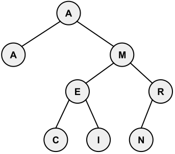
The root of the resulting tree is the node containing A. Our ACSL convention places duplicate keys into the tree as if they were less than their equal key. The tree has a depth (sometimes called height) of 3 because the deepest node is 3 nodes below the root. The root node has a depth of 0. Leaf nodes (nodes with no children) are: A, C, I, and N. Our ACSL convention is that an external node is a place where a new node could be attached to the tree. The final tree above has 9 external nodes. The tree has an internal path length of 15 (the sum of the depths of all nodes) and an external path length of 31 (the sum of the depths of all external nodes). To insert N (the last key), 3 comparisons were needed: against A (>), M (>), and R (≤).

To perform an inorder traversal of the tree, recursively traverse by first visiting the left child, then the root, then the right child. In the tree above, the nodes are visited in order: A, A, C, E, I, M, N, R. A preorder traversal (root, left, right) visits: A, A, M, E, C, I, R, N. A postorder traversal (left, right, root) visits: A, C, I, E, N, R, M, A. Inorder traversals are typically used to list contents in sorted order.

A binary search tree can support insert, delete, and search operations efficiently for balanced trees. In a tree with 1 million items, one can search for a particular value in about $\log_2 1{,}000{,}000 \approx 20$ steps. However, consider the binary search tree resulting from inserting A, E, I, O, U, Y in order — all letters land on the right side of A, making it very unbalanced.

To search for a node in a binary tree, the following algorithm is used:

p = root
found = FALSE
while (p ≠ NIL) and (not found)
  if (x < p's key)
    p = p's left child
  else if (x > p's key)
    p = p's right child
  else
    found = TRUE
  end if
end while

Deleting from a binary search tree:

p = node to delete
f = father of p
if (p has no children)
  delete p
else if (p has one child)
  make p's child become f's child
  delete p
else if (p has two children)
  l = p's left child
  r = p's right child
  make l become f's child instead of p
  stick r onto the l tree
  delete p
end if

These diagrams illustrate the algorithm. Left: delete I (0 children). Middle: delete R (1 child). Right: delete M (2 children).

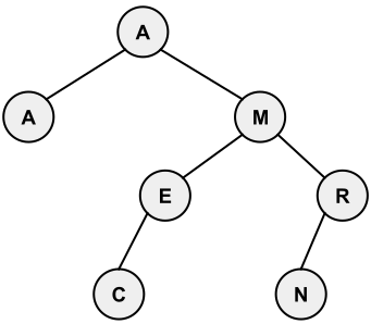
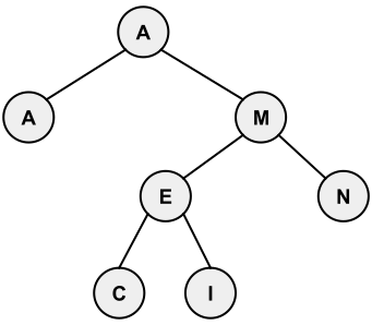
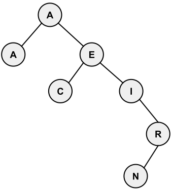
There are also general trees that use the same terminology but have 0 or more subnodes accessed with an array or linked list of pointers. Pre-order and post-order traversals are possible, but other BST algorithms do not apply. Applications include game theory, organizational charts, and family trees.

Balanced trees minimize searching time when every leaf node has a depth within 1 of every other leaf node. Complete trees are filled at every level and are always balanced. Strictly binary trees ensure that every node has either 0 or 2 children.

Priority Queues

A priority queue is quite similar to a binary search tree, but one can only delete or retrieve the smallest item. These operations can be done in time proportional to $\log_2 n$; retrieving the smallest item takes constant time.

The standard implementation uses a heap — a binary tree that maintains two properties: every node is less than or equal to both its children, and the tree has no “holes” (all levels are completely filled except the bottom level, which is filled left to right).

Insertion: place the new node at the bottom of the tree, then swap upward with its parent until the heap property holds. The heap below was built from AMERICAN (left), and the heap on the right shows the state after inserting C.

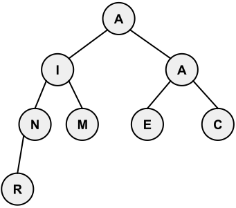
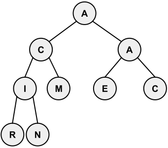
The smallest value is always the root. To delete it, replace it with the bottom-most, right-most element, then walk down swapping with the smaller child:

b = bottom-most and right-most element
p = root of tree
p's key = b's key
delete b
while (p is larger than either child)
  exchange p with smaller child
  p = smaller child
end while

When the smallest item is at the root, the heap is called a min-heap. A max-heap (largest item at root) is also common in practice.

Sample Problems

Problem 1

Consider an initially empty stack. After the following operations are performed, what is the value of Z?

PUSH(3)
PUSH(6)
PUSH(8)
Y = POP()
X = POP()
PUSH(X-Y)
Z = POP()

Solution: The first POP stores 8 in Y. The second POP stores 6 in X. Then 6 − 8 = −2 is pushed onto the stack. Finally, the last POP removes −2 and stores it in Z.

Problem 2

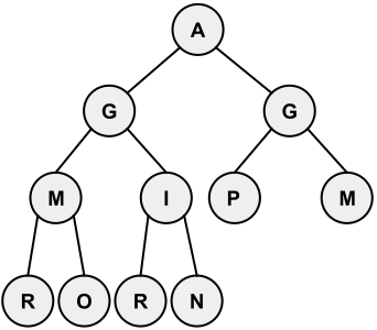
Create a min-heap with the letters in the word PROGRAMMING. What are the letters in the bottom-most row, from left to right?

Solution: The bottom row contains the letters RORN, from left to right. Here is the entire heap:

Problem 3

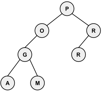
Create a binary search tree from the letters in the word PROGRAM. What is the internal path length?

Solution: P has depth 0; O and R have depth 1; G and R have depth 2; A and M have depth 3. Therefore, the internal path length is $2 \times 1 + 2 \times 2 + 2 \times 3 = 12$. Here is the tree:

Video Resources

ACSL Videos

The following YouTube videos show ACSL students and advisors working out some ACSL problems that have appeared in previous contests. Some of the videos contain ads; ACSL is not responsible for the ads and does not receive compensation in any form for those ads.

Other Videos